
Introduction
By their very nature, endowments and foundations face a unique challenge: balancing the conflicting goals of meeting current spending needs, as well as supporting long-term spending needs well into the future. The decision to spend now generally means that less money is available for future needs. Endowments and foundations generally have very long time horizons (perhaps infinite) and therefore can take a long-term perspective in determining an appropriate investment strategy. However, unlike other investors with long-term time horizons, such as young workers saving for retirement, endowment and foundation portfolios are meant to support annual withdrawals, for instance, to support college operating budgets, periodic building projects, grants to not-for-profit organizations, medical research, and other worthwhile projects. In a sense, endowments and foundations are akin to an individual who is in retirement for perpetuity.
We can help
A spending policy plays an important role in managing an endowment. We can help ensure yours is set up to balance the withdrawals needed to support your spending needs today while also growing your investments to sustain your mission for years to come. Schedule a call today to learn more about all of the ways we can help your organization.
Connect with usWhile choosing the appropriate spending rule is undoubtedly an important part of the investment management decision for endowments and foundations, asset allocation and investment management structure also have a major impact on whether these organizations are able to meet their goals. Invest too aggressively and the portfolio may be decimated by both spending and portfolio declines, but invest too conservatively and the portfolio may not provide sufficient growth to keep up with inflation. In general, asset allocation should be driven by time horizon, liquidity needs (i.e., spending or withdrawal requirements) and risk tolerance factors.
Key to the management of endowment/foundation assets is balancing the need for stability to meet current spending requirements with the pursuit of long-term growth to meet future obligations. As a result, we believe the ideal asset allocation would allow for meaningful exposure to fixed income securities, in line with a primary goal of providing income and stability of principal to meet on-going spending needs, but would also allow flexibility to increase exposure to equity securities in certain market environments in a manner consistent with the endowment/foundation’s long-term time horizon. Allowing for a range of equity exposure will provide for flexibility to adjust the portfolio’s exposure as economic and/or market conditions change. However, the first step in the management process for endowments and foundations is making the spending rule decision; as such, this paper will focus primarily on the various types of spending rules.
This paper is organized as follows: The first section discusses desirable characteristics of spending rules and presents several commonly used spending rules. The second section examines the performance of these spending rules over recent history, while the third section examines how spending rules would have held up in a stagflation environment (i.e., 1973-1982). The last section presents several conclusions from this analysis and several factors that we believe should be considered when determining spending rules. Throughout this paper, spending rules for a hypothetical college endowment are examined. However, the same general principles apply for other endowment types, as well as foundations.
Section 1: Spending Rules
A college endowment may support the college’s operating budget, scholarships for students, teaching positions, and periodic capital expenditures. In this context, the college relies on the endowment annually to help meet its expenses. Ideally, the level of annual support should keep up with inflation and for planning purposes there should not be large swings from year-to-year in the level of support. In addition to regular annual spending, a college endowment may support periodic capital expenditures, such as building projects, which may have dedicated fund-raising campaigns.
Endowments and foundations must have a methodology to determine how much to spend each year. There may be a minimum amount of spending required by certain foundations as a result of their tax-exempt status (e.g., private foundations). The determination of the yearly amount may be based on board discussions, weighing spending requests, or may involve formalized spending rules which determine annual spending based upon asset levels, inflation, prior year spending or some combination of these items.
Therefore, Trustees must decide on an appropriate spending policy and must decide how to invest the endowment’s portfolio. We believe characteristics of “good” spending rules include ones that:
- Allow an adequate amount of spending each year
- Have some degree of predictability from year to year
- Take into account inflation when applying the spending rule
- Allow spending to increase modestly during good times
- Maintain spending during difficult periods
- Do not spend so much that the portfolio declines on a real-basis.
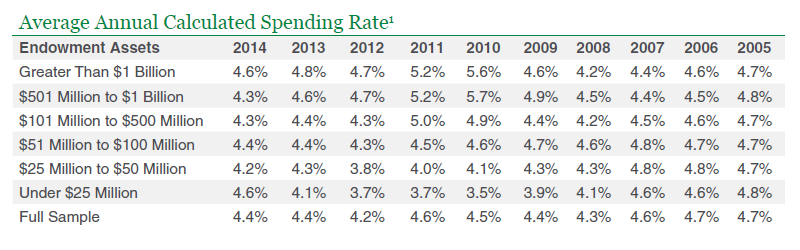
While there are myriad versions of spending rules across organizations, according to the 2014 National Association of College and University Business Officers (NACUBO) Endowment Study, the average annual spending rate was 4.4% over the 2014 calendar year. However, in past years average spending has been as high as 4.7% (2005 and 2006) and as low as 4.2% (2012). In forming any spending rule, an endowment/foundation should take into account factors such as endowment size, endowment payout as a percentage of total operating budget, need for income stability, portfolio risk, and relationship between restricted and unrestricted funds. Below we examine some of the more common spending rules typically utilized by many endowments and foundations. We examine the last three spending rules in further detail in various scenarios in Sections 2 and 3 of this paper.
Simple market value approach
Here, the idea is to merely spend a pre-specified percentage of the previous year-end market value (e.g., 5% of market value). This approach can lead to wide fluctuations in annual spending, depending on the performance of Plan assets and whether the market value of the assets goes up or down. Thus, in years when assets perform poorly, annual spending will be lower, and in years when assets perform well, annual spending will increase.
Average market value approach
Under this method, the annual spending rule is set at a certain percentage of a moving average market value (e.g., three-year average), sometimes with upper and lower limits. For example, such a spending rule may be specified as spending 5% of the moving three-year average of year-end asset values. A variation includes spending 5% of the moving three-year market value of assets but not less than 3% of current market value and not more than 7% of current market value. Such an approach attempts to smooth spending somewhat from year-to-year.
Inflation-adjusted approach
This approach takes current levels of inflation into account, and calls for spending an initial percentage of the portfolio’s market value, adjusting all withdrawals for inflation. In this way, spending is maintained on a real basis. For instance, an endowment may decide to initially spend 5% of assets, then each subsequent year spending is indexed by an appropriate inflation factor. A variation is that real spending (after inflation) should increase by 2% per year. Obviously, this will cause spending, in absolute terms, to be higher in years when inflation is higher, and vice versa. Therefore, this approach may also result in wide swings in annual spending, as withdrawals will vary based on portfolio performance and level of inflation.
Hybrid approach (Yale Rule)
Finally, a hybrid approach, as its name suggests, combines elements of all of these methods. Spending for a given year is generally composed of two parts: 1) a moving market value component, and 2) an inflation-adjusted component. As an example, a hybrid spending rule may state the amount to spend in a given year is one half of 5% of the three-year moving market value average plus one half of last year’s spending indexed by inflation. Further detail on the average annual spending rate for endowments from the 2014 NACUBO study are listed below.
Section 2: A Historical Perspective on Spending Rules
To gain a better understanding of these spending rules, let’s consider a hypothetical endowment, “XYZ Endowment,” and analyze spending and asset values over a specific period, January 1995 to January 2015. While full year returns for 2015 are not yet available, spending data based on the January 1, 2015 asset value is presented to illustrate the impact of recent market movements. The XYZ Endowment’s initial assets, initial spending, and asset allocation are as follows:
- $10 million dollars in assets on January 1, 1995;
- initially decided to spend $500,000 in 1995 (beginning of year withdrawal);
- has a 60% stock/40% bond asset allocation strategy, with annual rebalancing.
Now, we’ll examine spending and market values on a nominal and real basis for the period 1995-2015 under the three spending rule types. The spending rule parameters are given below.
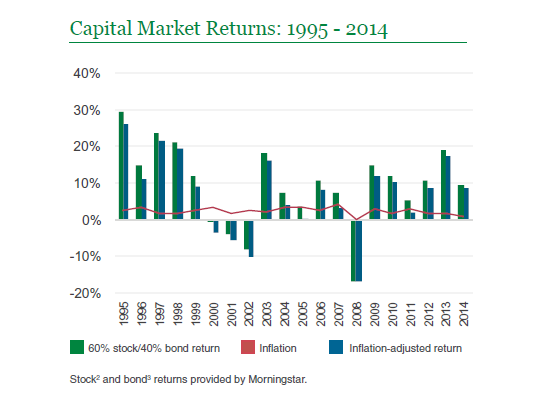
The investment return and inflation rate for each year from 1995-2014 are given in the Capital Market Returns chart at the top of the column to the right. This period is chosen to make the analysis current and also because it includes both bull market and bear market time periods. While the substantial market declines suffered in 2008 had a meaningful effect on year-end asset values, as we will see later, this period on the whole is comparatively benign from an inflation standpoint.
Under each of the three spending rules, 5% of the portfolio’s initial value (i.e., $500,000) will be withdrawn at the beginning of the first year. Under the percent of average market value approach (Rule #1), subsequent spending will only be dependent upon the portfolio’s nominal return, while under the inflation-adjusted approach (Rule #2), subsequent spending will depend only on annual inflation. The hybrid approach (Rule #3) takes into account both portfolio returns and annual spending.
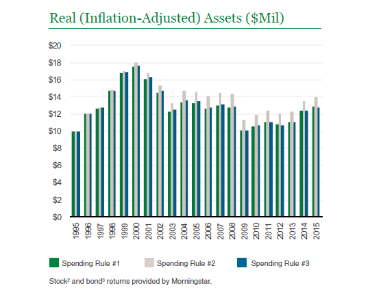
As the tables above illustrate, each of the three spending rules held up relatively well over the time period January 1995 to January 2008; under each spending rule both the real purchasing power of the portfolio and real annual spending were generally at least maintained. However, the effect of the bull markets and subsequent bear markets are noticeable under all three rules and especially during the recent downturn in 2008. For example, real assets climb from approximately $10 million to approximately $17 million in 2000 and then fall significantly to around $12 to $13 million in 2003. Real assets remain relatively stable, although levels differ by spending rule, ranging from approximately $12 to $14 million until the end of 2007, and then decline meaningfully to around $10 to $11 million by the beginning of 2009. Since 2009, real asset levels have recovered to different degrees depending on the spending rule. It is illustrative to examine spending under each of the three rules.
Rule #1: Percent of market value approach
5% of the three-year moving average of year-end assets, but not less than 3% of current market value and not more than 7% of current market value.
Under this rule, real spending may increase rapidly, but tends to readjust rapidly as well. Real spending increased during the period of strong portfolio performance in the late 1990s bull market. However, spending then decreased significantly to approximately $631,000 in 2005, a 22% decline from 2001, as the full effects of the bear market became reflected in the spending determination. Additionally, real spending decreased from 2008 to 2011 by 16% (from approximately $617,000 to $518,000), reflecting the meaningful declines in real assets during the most recent bear market. Withdrawal rates in terms of nominal assets ranged from a low of 4.3% in 1999, indicating that strong portfolio performance was not fully reflected in the spending determination, to a high of 5.8% in 2009, indicating that weak portfolio performance was not fully reflected in the spending determination. Overall, this moving-average market value approach has the effect of smoothing spending from year-to-year compared to an approach that simply calculates spending as a percent of the previous year ending market value, and generally results in the smallest fluctuation in the withdrawal percentage among the three approaches.
Rule # 2: Inflation-adjusted approach
Spend 5% of market value in the first year ($500,000), then index by inflation + 2%.
Under this approach, the dollar value of spending does not depend on portfolio returns, as real spending increases 2% per year regardless of portfolio performance. For example, despite the significant market declines in 2008, real spending gradually increased from approximately $643,000 in 2008 to $655,000 in 2009. Consequently, as the table on the previous page illustrates, of the three spending approaches presented, this approach has resulted in the most meaningful fluctuation in the withdrawal percentage. Specifically from 1995-2015 withdrawals varied from 3.1% to 5.8%, representing the largest degree of variation in absolute terms among the three spending approaches. Additionally, withdrawals increased from 4.5% of market value in 2008 to 5.8% in 2009 (the largest increase among the three spending approaches) even as inflation remained comparatively muted. Despite recent years of strong stock market performance, given that spending was not adjusted through periods of adverse market volatility in 2008, spending as percent of assets remains more elevated as of 2015 compared to other spending rules. Note that spending below a certain percent of assets may not be acceptable, due to tax requirements for certain types of foundations.
Rule # 3: Hybrid approach
Annual spending = part 1 + part 2. Part 1 = One half of 5% of the three-year moving average of year-end assets; Part 2 = One half of last year’s spending indexed by inflation.
With this spending rule, real spending generally increased (more slowly than in Rule #1) to approximately $778,000 in 2001, then receded (more slowly than in Rule #1) to approximately $551,000 in 2011. Reliance in part on last year’s spending indexed by inflation to determine the current year’s spending generally makes the actual annual dollar amount of real spending more predictable than spending under Rule #1. Overall, utilizing a hybrid spending rule typically results in a smoother real spending pattern than that observed with Rule #1 even though the actual withdrawal percentage may be more volatile.
Section 3: Stagflation Simulation
Examining how the various spending rules would have affected a hypothetical endowment’s spending and asset levels during certain economically significant periods of history is an important part of understanding the risks of the various spending rules. Specifically, periods of time in which the economy was in a recession, marked by sustained losses in the stock and/or bond market, or periods of high inflation, would have a significant effect on overall asset returns and levels of withdrawals. Examining how each of the aforementioned spending rules would have played out under this type of “economic stress testing” offers a glimpse of potential portfolio implications as economic conditions unfold in the future. Here, we take a look at one such historical time period, 1973-1982, which was marked by significant stock market losses against a backdrop of persistent, high inflation. For these scenarios, we utilize the same assumptions as in our prior example, including assuming a portfolio with a 60% stock/40% bond allocation.
Economic Environment
The early 1970s were typically characterized by rising inflation and high unemployment (i.e., stagflation). The National Bureau of Economic Research (NBER), which tracks economic cycles, records the economy as having entered a recessionary state in November 1973 that lasted through March 1975. Much of the blame for this recession is placed on an unexpected rise is oil prices. Around this time, GDP growth fell by approximately 3%, and unemployment jumped from 4.9% to a high of 9.0%. At the same time, the inflation rate peaked at 12.2% over the calendar year of 1974. The S&P 5002 fell by 14.7% in 1973 and 26.5% in 1974, before rebounding in 1975. As a result, this time period should prove useful for analyzing what would have happened to asset levels and spending withdrawals for a hypothetical endowment operating during this time.
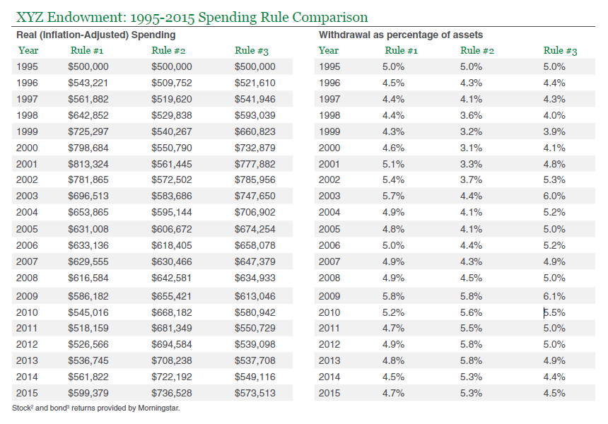
Percent of Market Value Approach
Under this methodology, the fund’s asset base would have declined by 28% in nominal terms and 41% in real terms from 1973 through the end of 1974 before rebounding in subsequent years and reaching $10.6 million (in nominal terms) in the beginning of 1982. Under this approach, spending levels would have tapered off in response to the falling market value of assets.
Specifically, spending would have fallen by 18% in nominal terms by 1976, and by 37% in real terms over the same time period. However, due to the effects of high inflation, real spending would have continued to fall in later years, reaching a 53% decline by the beginning of 1982. As expected, with the percent of market value approach, the withdrawal percentage would have risen from 5.0% in 1973 to 6.0% in 1975 before falling back to 4.4% in 1977, and subsequently rising to 5.1% in 1978 and 1979.
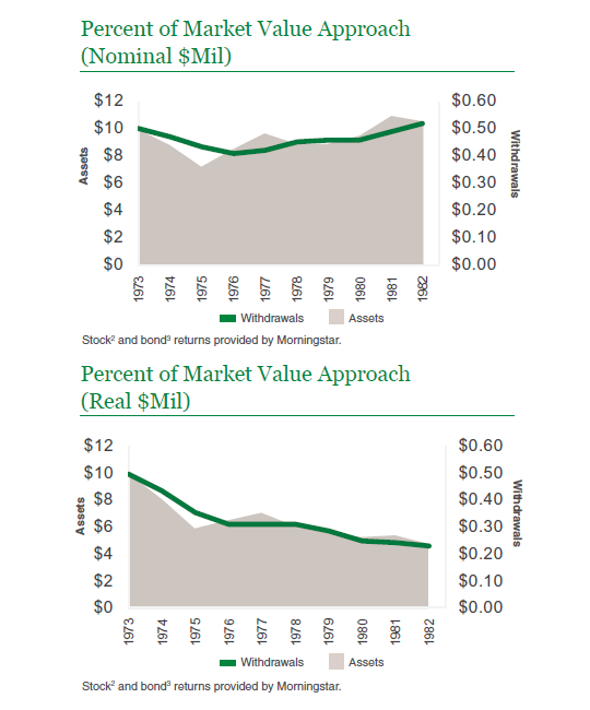
Inflation-Adjusted Approach
With this spending rule, assets would have fallen by a similar 28% in nominal terms and 41% in real terms from 1973 through 1974. However, because of the higher levels of withdrawals experienced with this approach, nominal and real assets would continue to decline even as the stock market recovered after the bear market, falling by 34% in nominal terms and 70% in real terms by the beginning of 1982. This would leave the portfolio with only $6.6 million in nominal assets by the beginning of 1982.
Because of the inflation-adjusted nature of this spending rule, the nominal amount withdrawn from the endowment would have increased by 160% ten years later at the beginning of 1982. However, the real withdrawal amounts would have been substantially less, due to the effects of inflation, increasing by only 18% by the beginning of 1982. The withdrawal percentage would have been highest under this spending rule, steadily increasing from 5.0% in 1973 and reaching a staggering 19.6% of assets by the beginning of 1982.
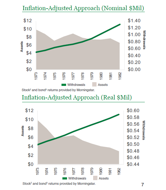
Hybrid Approach
Under the hybrid spending rule approach, nominal assets would have fallen by 28% by 1974 before rebounding in later years, reaching $10.1 million at the beginning of 1982. In real terms, however, assets would have continued to fall, reaching a depletion level of -54% by the beginning of 1982. Nominal withdrawals would have remained the most constant under this spending rule, falling slightly, by 9% by 1977, before rebounding by 6% by the beginning of 1982. Real withdrawals, however, would have fallen by 33% in 1977 and by 52% by the beginning of 1982. The withdrawal percentage under the hybrid approach would have risen to 7.0% by 1975 before falling back down to 4.8% in 1977 and hovering at a roughly 5% level thereafter.
Section 4: Conclusions
As the historical scenarios have indicated, the various spending rules have differing impacts on total assets and overall spending. As we have seen, choosing an inflation-adjusted approach results in higher levels of both nominal and real spending, while the percent of market value approach generally results in the lowest level of spending. As might be expected, the hybrid approach tends to fall somewhere in between, typically with a more predictable level of spending resulting from year-to-year. It follows then, that in a high inflation environment the inflation-adjusted approach also requires the largest percentage withdrawals from the portfolio, followed by the hybrid approach, with the percent of market value rule requiring the smallest percentage withdrawals.
When deciding on a spending rule, endowments and foundations must consider their current and future goals and needs. A good spending rule is one that will allow for an appropriate level of spending each year, allows for relatively stable and predictable spending from year-to-year, regardless of whether the portfolio is experiencing positive or negative returns, and that will support spending well into the future, in line with an endowment or foundation’s long-term focus. Such a spending rule may also take inflation into consideration, to ensure that annual spending does not decline on a real basis. The “correct” spending rule may vary from institution to institution, depending on the specific goals and objectives of each endowment or foundation. However, we believe taking each of these aforementioned factors into account will help to ensure that the chosen spending rule remains consistent with the organization’s needs.
We believe two of the most important decisions that the spending rule will help to drive are the asset allocation and investment manager decisions. In addressing the unique needs of endowments and foundations, it is of utmost importance to consider the manner in which such an organization’s assets are spread across asset classes. Studies have shown that asset allocation is by far the largest determinant of variability in portfolio returns4. As such, Trustees should give careful consideration to the asset allocation decision, including how assets are distributed amongst multiple investment managers.
To provide historical perspective on the importance of the asset allocation decision and the potential volatility associated with various levels of equity exposure, we can examine market return data over the past 89 years.
While historical data shows an increased equity allocation generally improves the chances for long-term capital appreciation, increasing equity exposure also increases the probability of experiencing sustained declines. For example, while a mix of 60% stocks and 40% bonds provided an 8.8% annualized return over the period from 1926-2014, this allocation experienced losses in approximately 21% of the rolling one-year periods and 5% of the rolling five-year periods over the 89 years for which data is available. Likewise, the minimum and maximum returns for rolling time periods have also varied dramatically. For example, the maximum annualized return for a mix of 60% stocks and 40% bonds over a five-year rolling time period was 24.6%, whereas the minimum annualized return over a five-year rolling time period was -7.8%. History has clearly shown that meaningful exposure to equities may lead to extended periods of market value declines, which can lead to rapid portfolio depletion for a portfolio potentially facing significant ongoing withdrawals.
There is a clear trade-off between pursuing long-term growth through equity exposure and maintaining stability to meet ongoing withdrawal requirements, with increased exposure to stocks historically providing higher returns, but also increased capital risk. When identifying an appropriate asset allocation for a portfolio, this trade-off should be considered in light of long-term investment objectives.
Likewise, no single (i.e., static) mix of asset classes can be expected to meet an investor’s investment goals in all environments. That is, the idea of basing asset allocation decisions solely on historical risk/return relationships is similar to driving a car by looking in the rear-view mirror rather than the road ahead. A passive approach to asset allocation does not recognize a need to consider current conditions. In short, a passive approach generally relies on long-term history as a guide, while an active approach allows for decisions in light of today’s environment. Implemented successfully, an active approach should allow for a shift out of over-valued market segments prior to a decline, while a passive approach would advocate a constant allocation despite valuation levels. For example, today’s historically low interest rate environment suggests that fixed income markets may have difficulty providing returns in line with their long run historical averages over the next several years. Thus, it is vitally important for endowments and foundations to incorporate a mechanism for actively adjusting their asset allocation on an ongoing basis, in response to current market conditions. Taking an active approach to the asset allocation decision, in conjunction with crafting a carefully defined spending rule, can help endowments and foundations to meet their goals of balancing stability of returns with their need for long-term capital growth.
In summary, careful consideration is warranted when choosing a spending rule to direct withdrawals for any foundation or endowment. A close examination of the specific organization’s goals, objectives, and needs is warranted as both an initial and ongoing part of this process. Insofar as the spending rule decision helps to drive the subsequent asset allocation and investment manager structure decisions, we believe this can be one of the most important and pressing choices a Board of Trustees or Investment Committee makes.
Analysis by Manning & Napier. Source: Morningstar. © Morningstar 2015. All rights reserved. The information contained herein: (1) is proprietary to Morningstar and/or its content providers; (2) may not be copied, adapted or distributed; and (3) is not warranted to be accurate, complete or timely. Neither Morningstar nor its content providers are responsible for any damages or losses arising from any use of this information, except where such damages or losses cannot be limited or excluded by law in your jurisdiction. Past financial performance is no guarantee of future results.
12014 NACUBO Endowment Study. 832 institutions provided spending rate information for the 2014 fiscal year. Table data are equal-weighted. Institutions have the opportunity to report ten years of spending rate data in each year’s survey.
2Stock data is reflective of the S&P 500 Total Return Index (S&P 500), which is an unmanaged, capitalization-weighted measure of 500 widely held common stocks listed on the New York Stock Exchange, American Stock Exchange, and the Over-the-Counter market. The Index returns assume daily reinvestment of dividends and do not reflect any fees or expenses. S&P Dow Jones Indices LLC, a subsidiary of the McGraw Hill Financial, Inc., is the publisher of various index based data products and services and has licensed certain of its products and services for use by Manning & Napier. All such content Copyright ©2015 by S&P Dow Jones Indices LLC and/or its affiliates. All rights reserved. Neither S&P Dow Jones Indices LLC, Dow Jones Trademark Holdings LLC, their affiliates nor their third party licensors make any representation or warranty, express or implied, as to the ability of any index to accurately represent the asset class or market sector that it purports to represent and none of these parties shall have any liability for any errors, omissions, or interruptions of any index or the data included therein.
3Bond data is reflective of the Ibbotson Associates SBBI U.S. Intermediate-Term Government Bond Index, which is an unmanaged index representing the U.S. intermediate-term government bond market. The index is constructed as a one bond portfolio consisting of the shortest-term non-callable government bond with no less than 5 years to maturity. The Index returns do not reflect any fees or expenses.
4Determinants of Portfolio Performance; Brinson, Hood, Beebower; Financial Analysts Journal; 1995.